Computer vision opens the way to many business opportunities. In this multi-part blog series, we will show how ML teams can use lossy image compression to improve their computer vision models. In Part 1, we see how we can compress training images to reduce the volume of physical storage required without sacrificing model performance. Given a fixed starting volume of physical storage, the compression of training data frees up physical storage (or equivalently money) for other uses. In Part 2, we see how we can re-appropriate this newly vacated storage space to additional compressed image training data, resulting in improved model performance at the same original physical storage capacity (and equivalently dollar budget). 

Let's dive in!

State-of-the-art computer vision models require a large volume of image data, and images can be expensive to store. For many machine learning teams, data storage budgets implicitly limit the number of images that engineers can use to train their models, and these constraints result in up to 70% of newly created data being archived or deleted [1]. Machine learning groups will need to adopt new strategies to take advantage of the ever-growing image data potentially available to build the best models.

Compressing images can help solve the data storage challenge. Compression can significantly reduce the amount of physical storage required for a given set of images, freeing space for additional training observations. However, if we constrain ourselves to lossless compression—where you can reconstruct the image exactly—storage gains are limited. Losslessly compressed images are typically about half the original file size for photographic images. If we allow for some loss in a way that does not affect model performance, we can compress images significantly more, potentially to a few percentage points of their original file size.

The limitation to lossy compression is that the image quality is degraded. We can measure the perceived change in image quality with a perceptual distance measure between images, such as the Butteraugli distance. Some image codecs, such as JPEG XL, allow us to compress to an approximate Butteraugli distance, discarding as much file size as possible given the allowed degradation.  

As an illustrative example, consider the following image of risotto, which was originally stored as a high quality JPEG. 

We can compress the image to a Butteraugli distance of 2 from the original image using JPEG XL, giving the following image:

And, finally, compressing the image to a more extreme Butteraugli distance of 10:

At this distance, we begin to see square-like artifacts, and the image looks considerably degraded. 

The greater the distance, the more the image is compressed and the lower the file size. To measure how much we have compressed with respect to file size, we define the data compression rate:

\(DCR = 1 - \frac{\text{Compressed Size}}{\text{Uncompressed Size}}\)

A larger DCR indicates a smaller file size. By testing the compression on sample images originally stored as JPEGs, we see that DCR increases quickly as the Butteraugli distance increases.

JPEG is already a lossy image compression format. Despite this fact, we can significantly compress the image file size relative to its previously-stored JPEG size using more modern techniques such as JPEG XL. The left y-axis shows the DCR relative to the JPEG format. The right y-axis shows the DCR relative to the uncompressed image size, where the gains are much higher.   

If we were instead to use a lossless image compression format like PNG, we would only compress the image by 53%, compared to the >90% data compression rate we achieve with JPEG and JPEG XL.  

While we may only need to tolerate a small amount of perceptual degradation to the image to achieve a significant compression ratio, machine learning engineers need to know how compressed training images affect computer vision models.

The impact of compression for machine learning is not immediately clear. On one hand, image compression algorithms are discarding data that could potentially be important to machine learning models (even if it's not important to the human eye). On the other hand, image compression algorithms throw away high frequency "noise" components of the image, potentially helping the machine learning to attend to the most important information. 

Image Classification on Compressed Images

Image classification is a fundamental computer vision task—given an input image, we assign a label within a certain number of possibilities (‘classes’). We begin to investigate the question of how compressing training data impacts machine learning models using a simple image classification task. 

Dataset: The Food101 dataset has 75,750 training images and 25,250 test images, one of which is the risotto image shown previously. Each image belongs to one out of 101 possible classes ranging from beignets to prime rib. Classes are balanced in both the training and the test sets. Images are originally stored as JPEGs.

Task: Identify what type of food is shown in a given image. 

Model: We use a Vision Transformer that has been pre-trained on ImageNet to perform this task (Base Model). We fine-tune the model on the Food101 training set for 3 epochs.

Evaluation Metric: We use accuracy, defined as the fraction of images that are assigned the correct class.

We fine-tune eleven models, one using the uncompressed data and the other 10 using training images compressed to Butteraugli distances 1 through 10. We evaluate each model 11 times, once on the uncompressed test set and on the test set compressed to distances 1 through 10. The resulting output gives us performance values on a grid of test and train compression levels. 

In the following plot, we illustrate the models’ performance relative to a model that is both trained and evaluated on uncompressed data. For each point, we calculate the current model ‘s accuracy divided by the uncompressed accuracy – the percentage of the uncompressed performance. Higher numbers indicate closer to the original performance. The circles represent the observed accuracies, and the background is a 2-dimensional linear interpolation of the observed data. 

Compressing has minimal impact on prediction accuracy until we compress the image to very high levels, beyond around 70%. The model seems to be more sensitive to test set compression than to training data compression.

To illustrate that this is not purely an artifact of the ViT model, we use a different architecture to replicate the results. 

Model: We use a linear classifier layer on top of SwAV features generated with a ResNet-50 architecture. All weights except the final classification layer are frozen during training.

Once again, we see that we can compress the training set by more than 60% before classifier accuracy degrades significantly. With this architecture, the model seems more sensitive to highly compressed training data, but this effect is only clear for compression rates above 70%.

Object Detection on Compressed Images

In our demo models, compressing images largely doesn't impact image classification accuracy.  However, image classification is a relatively easy computer vision task. Does the same hold for more complex tasks, such as object detection? 

Dataset: We use the PASCAL VOC 2012 dataset, which contains 20 classes, 5,717 training images, 5,823 validation images, and 27,450 labeled objects. The images are originally stored as JPEGs. 

Task: Identify objects with bounding boxes and assign them to one of the 20 potential categories. 

Model: We use a Faster R-CNN model with a ResNet-50 backbone that has been pre-trained on ImageNet (MMDetection R-50-FPN 1x). 

Evaluation Metric: We use the PASCAL VOC challenge metric, the mean average precision  (mAP). This metric considers different definitions of a positive prediction and also averages across classes. For a more detailed description of the PASCAL VOC metrics, please see other resources such as this article.

For this task, we train an additional model at a Butteraugli distance of 0.5 to provide more information on lower compression levels. 

For this task, it seems that the evaluation accuracy depends primarily on the test set compression level, whereas the model training set compression level has little impact on accuracy.

Semantic Segmentation on Compressed Images

Another important task in computer vision is semantic segmentation, where every pixel of an image must be assigned to a class. Given the pixel-level classifications, semantic segmentation is a challenging computer vision task. To test the impact of compressed images on segmentation tasks, we employ the following setup. 

Dataset: The Cityscapes dataset contains 5,000 images with fine annotations for semantic segmentation. The images are originally stored as PNGs. 

Task: Given an image, assign one of 19 labels to each pixel, segmenting each region of the image into a particular class.

Model: The model is a Segformer with a pre-trained encoder trained on ImageNet 1k, specifically the Nvidia mit-b5.

Evaluation Metric: Mean intersection over union (mIoU) is an evaluation metric that calculates the IoU for each class and then averages across classes. A second metric is mean accuracy (mAcc), which requires calculating the per-class accuracy, then averaging across classes.

Note that the original images for the Cityscapes dataset are stored as PNG files, so the DCR is much higher in this case. We focus our analysis on Butteraugli distances of 1 or greater to see greater detail. First, we see the mean intersection over union.

The models can be trained on data compressed by 97% —requiring just 3% of the original training data storage—without significant degradation in this metric. We repeat the analysis for the mean accuracy.

Once again, we see a similar pattern that compression has little effect on model performance until the highest levels of compression.

Intuition: Why Compression has Limited Impact on Computer Vision Tasks

Somewhat surprisingly, even substantial compression seems to have minimal impact on computer vision tasks. Can we understand why AI models training is robust to compression artifacts? 

When images are compressed in a lossy way, image codecs tend to discard the least perceptually important information first. In other words, image quality is degraded as little as possible for a given amount of information loss. Given the human visual processing system, the least important information is typically color and high frequency features.

Machine learning models may not rely heavily on this information either. To test this hypothesis, we will test how sensitive the image classification model is to changes in different frequencies in the image. To explain our method, we begin with a brief digression into how JPEG and JPEG XL stores images. 

JPEG and JPEG XL Image Storage

JPEG and JPEG XL are two image codecs that rely on similar basic strategies to compress image data. The first stage of encoding an image is to change the color space from the familiar RGB representation to another color space called YCbCr. The Y channel, called the “luminance,” roughly captures the brightness of components of the image. The Cb and Cr channels are two different “chrominance” channels that capture the hue of the image. 

Both JPEG and JPEG XL typically downsample the chrominance channels, taking advantage of the fact that humans are less sensitive to color—often estimated to be a third as sensitive as we are to luminance changes [2]. 

Given this new representation of the image, the image is broken into 8 pixel by 8 pixel squares for each channel. Each patch is then deconstructed using a Discrete Cosine Transform (DCT). Images can be represented as a combination of different frequency components. The DCT uses the following basis of 64 different frequencies to represent the image. 

For each 8 by 8 pixel square, we will end up with 64 coefficients – one for each DCT basis block. We can reconstruct the original square by multiplying each block by the corresponding coefficient and summing across all 64 blocks. 

The advantage of this representation is that we can be less precise with storing the coefficients for higher frequency basis blocks (the lower right) because humans tend to be less sensitive to high frequency changes in images. By being less precise with how we represent these coefficients, we can save significantly on file storage space. For JPEG and JPEG XL, coefficients for the lower right-hand corner of the DCT coefficients are rounded more aggressively (in a process called quantization), whereas the coefficients in the upper left hand corner are stored with the greatest precision. Different levels of compression discard more or less information in this stage.  The more aggressive the rounding, the more information is discarded, thus saving more storage space.

Testing Model Sensitivity to Perturbations of Different Frequencies

With this knowledge of how images are stored, we have additional tools to measure how sensitive our machine learning models are to changes in information at different frequencies – such as the changes induced by compression. 

For a given image, we can perturb the coefficient on a single DCT coefficient, changing the image slightly by increasing the prevalence of a single frequency in a given block. This is quite similar to what happens in the quantization stage of image compression, discarding some of the precision for different frequencies. With this new, slightly altered image, we can then test how much a machine learning model’s prediction changes as a result of this perturbation. 

In our analysis, we are only perturbing one DCT coefficient at a time. However, these changes can be difficult to see. To get a sense for what these changes to the image might look like in terms of visual impact, we perturb all blocks in the following example image of foie gras from the Food 101 dataset. For model evaluation, these changes would only impact one 8 pixel by 8 pixel region in the image. 

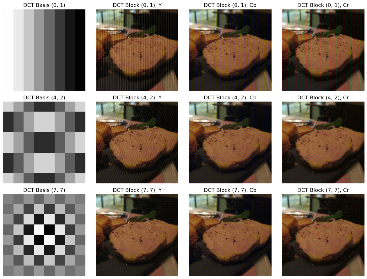
As perceptual studies suggest, the perturbations to the lower frequency components (first row) are more easily perceived than the perturbations to the higher frequency components (last row).

We repeat these perturbations for a sample of \(n\) = 32 images sampled from our Food101 test data set. We evaluate an image classification model (trained on uncompressed data) on the original unperturbed image and each of these perturbed images. We then can measure the change in prediction,

Where \(\varepsilon_{DCT(b,i,j)}\) is the perturbation to block \(b\)’s \(i,j\)’th DCT coefficient. Essentially, \(\Delta_{i,j}\) approximates the average gradient of our prediction probabilities in the direction of the given frequency component.

By calculating \(\Delta_{i,j}\) for each of the DCT basis blocks and each color channel, we can determine how much the model predictions change—that is, how sensitive the model is to changes in that frequency component for that color channel. 

Running this test on a sample of 32 JPEG images from the Food101 dataset and using the image classifier trained on uncompressed images, we obtain the following results. 

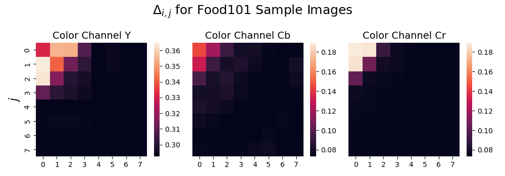
As we anticipated, the model is less sensitive to perturbations to the higher frequency DCT coefficients. This finding provides evidence that machine learning models may be less sensitive to compression artifacts in images because they do not depend on the high frequency information that compression discards to make their predictions. 

Overall, we find that in many common computer vision applications, training images can be compressed without significant impact to model accuracy. Models seem to be relatively insensitive to the changes in the high frequency information caused by compression, providing evidence for this robustness. Different tasks may necessitate different levels of compression based on the requisite accuracy, but it is worth considering compressing images beyond PNG or JPEG, as we can save significantly on storage costs with little impact to our computer vision models.

Subscribe to our newsletter below to be notified about Part 2, where we show how model accuracy improves when we apply those compression-related storage savings to additional training data. In effect, we show how a greater number of compressed images can improve model performance given a fixed data storage budget. Stay tuned!

And leave a message in the comments if you'd like to see a similar analysis for other model architectures or tasks.

[1] Deloitte. (2022). AI and data management: A $20 billion opportunity. https://www2.deloitte.com/us/en/insights/industry/technology/ai-and-data-management.html 

[2] https://en.wikipedia.org/wiki/Chroma_subsampling